
#> @rounds: number of rounds or matches in one game
#> @prob: probability of betrayal and cooperation
#> @choice: first choice to start the game. Choice inversion will be applied if staring choice = 1
#> @replace: sampling with replacement based on choice order. A vector of length 2

tit.for.tat <- function(rounds,
                        prob,
                        choice,
                        replace = TRUE,
                        ...){

  # Check arguments
  stopifnot({
    is.integer(rounds)
    is.double(prob)
    is.logical(choice)
    is.logical(replace)
  })

  choice_order <- c(choice, 1 - choice)
  p1 <- logical(rounds)
  p2 <- logical(rounds)


  p1[1] <- choice
  p2[1] <- TRUE

  for (i in 2:rounds) {
    if (choice_order[1] == TRUE) {
      inv.prob <- c(prob[2], prob[1])
      p1[i] <- sample(choice_order, size = 1, replace = replace, prob = inv.prob)
    } else {
      p1[i] <- sample(choice_order, size = 1, replace = replace, prob = prob)
    }

    p2[i] <- p1[i - 1]
  }
  result <- list(P1 = as.numeric(p1),
                 P2 = as.numeric(p2))
  return(result)
}

table(tit.for.tat(200,prob = c(.459,.237), choice = 0, replace = T))
#>    P2
#> P1   0  1
#>   0 85 47
#> 1 47 21not so quickly!
Recently, I become intrigued by game theory algorithms, not because I absolutely love playing games, but because it offers a quantifiable, systematic way to understand human relationships. I find the certainty of science and systematization reassuring to some degree so when I learned about this game called “the prisoner’ dilemma”, I thought it would fun to experiment and figure out the answer to this classic scenario. This game’s solution extends beyond hypothetical situations, addressing questions like: What’s the best strategy for handling conflict in various contexts—be it a card game, a business deal, or interpersonal relationships? Should we always cooperate and risk betrayal?
In his landmark work, R. Axelrod1 said:
1 The Evolution of Cooperation. Basic Books, Inc. New York, 1984
The Cooperation theory [here] is based upon an investigation of individuals who pursue their own self–interest wihtout the aid of central authority to force them to cooperate with each other. The reason for assuming self–interest is that it allows an examination of the difficult case when cooperation is not completely based upon a concern for others or upon the welfare of the groups as a whole.
I’ve heard the phrases “Meet in the middle”, “always compromise” or “never split the difference” but they all seem either idealistic or downright selfish. In a high-stakes situation, should we always cooperate? Yes or not so quickly!?.
the prisoner’s dilemma
Let the prisoner’s dilemma answer these questions for us.
The iterated version of the dilemma was presented as a hypothetical scenario by R. Axelrod:
Two bank robbers happen to meet. They decide to pull a job together. The cops nab them, but without enough evidence to convict. They need a confession. And they know both robbers are unlikely to talk, since if neither implicates the other, the cops can keep them in jail for only 30 days.
So they put the two in separate cells. They go to the first prisoner and say: “If you rat on your partner and he stays mum, we’ll let you go and he’ll do ten years.If you both rat on each other, you’ll both do eight years.” Then they go to the second prisoner and say the same thing.
The first prisoner thinks it over. “If he rats on me and I don’t rat on him, then I lose big-time. If I rat on him and he doesn’t rat on me, then I win big-time. Either way, the smart move is to rat on him. I’ll just hope he’s a sucker and doesn’t rat on me.” The second prisoner reasons the same way. So they rat on each other, and the cops get their two convictions. If the prisoners had cooperated, both would have gotten off easy. Instead, the rational pursuit of self-interest has put them both in a world of pain.
To win the game, at least one player must cooperate in the face of betrayal, otherwise both contestants would face unfavorable outcomes.
the rules
The rules of the iterated prisoner’s dilemma:
- Two players play 200 matches against each other and against an algorithm that betrayed or cooperated at random.
- Players obtain three points for mutual cooperation, one for a mutual betrayal, and five for the player who betrays when the other cooperates.
the path to follow
I’ll attempt to provide four solutions to this problem. The first algorithm will never be the first to betray and will copy the opponent’s previous choice. The second solution will betray in response to a cooperation five percent of the time; the third solution will not cooperate first and then imitate each of player 1’s choices, and the last one will never betray first, but will retaliate in turn on every remaining move until the end of the game.
The official winning strategy was the following:
- In the first match-up, cooperate.
- In every match-up after that, do what the opponent did in the preceding match-up.
the tit–for–tat solution
I’ll imitate this strategy in the first algorithm.
First,I’ll create a function for player 2 that chooses to cooperate on the first attempt, and copies player 1’s previous choice on subsequent moves. To do this, I have to iterate over each of player 1’s choices, and store player 2’s replies in a new vector.
To determine the choice order I’ll create a vector of length 2 with player 1’s original choice and subtract 1 from that choice to obtain the alternative. To create the vector of choices of length \(n\), I’ll append player 1’s original choice to a vector of length \(n-1\) ensuring that the first choice is always in position 1 p1[1]. The resulting vector will be of length n.
We’ll make a vector or player 2’s choices of length \(n\) equal to p1. The first choice will always be cooperation, and all subsequent choices will be player 1’s previous response p1[ i -1].
Always remember to initialize vectors and perform operations outside the loop, if possible. Doing this will sometimes make your function much, much faster.
the backstabber prober (bsp)
The only difference between Tit–for–Tat and the BSP2 is that we’re adding a random component that will cause player 2 to betray player 1 after a cooperation. Player 2 will always cooperate on the first round, but the algorithm will be less predictable than the previous one. I may be wrong, but I think this one will not do as well as Tit–for–Tat.
2 This strategy follows the Joss strategy featured in the 1984 book by R. Axelrod.
3 Under the uniform distribution, every outcome is equally likely to occur so we should see outcomes less than .05 occur less than 5% of the time.
To implement the random component needed to defect on 5% of cooperative responses, I will identify each time player 1 chooses to cooperate and then defect when randomly generated number from the uniform distribution is less than or equal to .053. If the randomly generated number is greater than my default, I’ll revert back to the tit–for–tat strategy.
#> @prob: probability of betrayal and cooperation
#> @default: percentage of cooperative responses on which player 2 betrays player 1

prober <- function(rounds,
                   prob,
                   choice,
                   default,
                   replace = TRUE,
                   ...){

   # Check arguments
  stopifnot({
    is.integer(rounds)
    is.double(prob)
    is.logical(choice)
    is.double(default)
    is.logical(replace)
  })

  choice_order <- c(choice, 1 - choice)
  p1 <- logical(rounds)
  p2 <- logical(rounds)

  p1[1] <- choice
  p2[1] <- TRUE

  for (i in 2:rounds) {
    if (choice_order[1] == TRUE) {
      inv.prob <- c(prob[2], prob[1])
      p1[i] <- sample(choice_order, size = 1, replace = replace, prob = inv.prob)
    } else {
      p1[i] <- sample(choice_order, size = 1, replace = replace, prob = prob)
    }

    if (p1[i - 1] == TRUE) {
      if (runif(1) < default) { # % chance to betray after cooperation
        p2[i] <- FALSE
      } else {
        p2[i] <- TRUE
      }
    } else {
      p2[i] <- p1[i -1]
    }
  }
  result <- list(P1 = as.numeric(p1),
                 P2 = as.numeric(p2))
  return(result)
}

table(prober(200,prob = c(.459,.237), choice = 0, default = .05, replace = T))
#>    P2
#> P1   0  1
#>   0 68 48
#>   1 51 33
the corteous cat
A less creative but more common solution is to simply emulate each of player 1 moves. Player 2 will never cooperate first unless player 1 chooses to cooperate. This copy cat algorithm is looking at the current round and not concerned with the previous moves.
copy.cat <- function(rounds,
                   prob,
                   choice,
                   replace = TRUE,
                   ...){

 # Check arguments
  stopifnot({
    is.integer(rounds)
    is.double(prob)
    is.logical(choice)
    is.logical(replace)
  })

  choice_order <- c(choice, 1 - choice)
  p1 <- logical(rounds)
  p2 <- logical(rounds)

  p1[1] <- choice
  p2[1] <- FALSE

  for (i in 2:rounds) {
    if (choice_order[1] == TRUE) {
      inv.prob <- c(prob[2], prob[1])
      p1[i] <- sample(choice_order, size = 1, replace = replace, prob = inv.prob)
    } else {
      p1[i] <- sample(choice_order, size = 1, replace = replace, prob = prob)
    }

    p2[i] <- p1[i]
  }
  result <- list(P1 = as.numeric(p1),
                 P2 = as.numeric(p2))
  return(result)
}

table(copy.cat(200,prob = c(.459,.237), choice = 0, replace = T))
#>    P2
#> P1    0   1
#>   0 140   0
#>   1   0  60
the squirrel’s revenge
The last algorithm will play nice on the first round but will exact revenge on player 1 until the end of the game4.
4 A copy of the aggressive Friedman’s algorithm.
The key to achieve such vengeful results is to track when player 1 switches from betrayals to cooperation. Once we identify a betrayal, player 2 will no longer cooperate. I’ll add one argument zero_switch to identify when player 1 chooses to defect, causing player 2 to defect on every move for the remainder of the game.
We have to pay careful attention to the choice probability here; if the probability of betrayal is higher than cooperation, the revenge algorithm will most likely never cooperate after the first few rounds. This player is a more revengeful fellow. Let’s see how to implement it.
exact.revenge <- function(rounds, prob, choice, replace = TRUE,...) {
  # Check arguments
  stopifnot({
    is.integer(rounds)
    is.double(prob)
    is.logical(choice)
    is.logical(replace)
  })

  choice_order <- c(choice, 1 - choice)
  p1 <- logical(rounds)
  p2 <- logical(rounds)

  p1[1] <- choice
  p2[1] <- TRUE

  zero_switch <- FALSE

  for (i in 2:rounds) {
    # Generate player 1's move
    if (choice_order[1] == TRUE) {
      inv.prob <- c(prob[2], prob[1])
      p1[i] <- sample(choice_order, size = 1, replace = replace, prob = inv.prob)
    } else {
      p1[i] <- sample(choice_order, size = 1, replace = replace, prob = prob)
    }

    # Player 2's response
    if (p1[i - 1] == FALSE) {
      zero_switch <- TRUE
    }
    p2[i] <- ifelse(zero_switch, FALSE, TRUE)
  }
  result <- list(P1 = as.numeric(p1),
                 P2 = as.numeric(p2))
  return(result)
}

table(exact.revenge(200,prob = c(.159,.437), choice = 1, replace = T))
#>    P2
#> P1    0   1
#>   0  53   1
#>   1 145   1
algorithm face off
Now that all four algorithms are created, we need a function to evaluate the overall performance in total points after 200 rounds.
First, we need an outcome matrix to store the outcome of each choice combination. Then, I have to create a function that repeatedly compares algorithms over n number of games. To do this, I will update the choice order for each game, if necessary; store total number of choices per game in two vectors, one for each player, create a list and evaluate choice outcome against the outcome matrix, and then sum each player’s score in the new list to find the total number of points per game. Finally, I would have to calculate the average number of total points per game and compare the algorithms.
However, not every algorithm takes the same list of arguments. The prober algorithm requires a default that is not specified anywhere else, and I must implement a comparison function that will take a default probability but only apply it to one of the algorithms no matter its order in the list. To do this, I’ll check each argument entered in the function and create two lists, one for the prober algorithm and a second for the second algorithm. The first list will contain the default argument and, if there’s a value specified, apply it to prober, the second will only take a default probability if the algorithm requires a default.
#> arguments include:
#>  @alg: algorithms to compare
#>  @rounds: number of rounds in a game
#>  @prob:   probability of betrayal and cooperation.
#>  @choice: starting choice.
#>  @default: percentage of cooperative responses on which player 2 betrays player 1
#>  @iter: how many games of `n` rounds should be played.

comp.alg <- function(alg,
                     iter = NULL,
                     rounds,
                     prob,
                     choice,
                     replace = TRUE,
                     default = NULL){
  #Check arguments
  stopifnot({
    is.list(alg)
    is.numeric(iter) && iter > 0})

  out <- matrix(c(3,5,0,1), nrow = 2, byrow = TRUE)
        rownames(out) <- c("P1.C","P1.B")
        colnames(out) <- c("P2.C","P2.B")

create.args <- function(func,common_args, default){

  fun_args <- names(formals(func))
  args <- common_args[names(common_args)%in% fun_args]
  if("default" %in% fun_args && !is.null(default)){
    args$default <- default
  }
  args
}

common_args <- list(rounds = rounds,
                        prob = prob,
                        choice = choice,
                        replace = TRUE)

p1_args <- create.args(alg[[1]], common_args, default)
p2_args <- create.args(alg[[2]], common_args,default)

  play.game <- function(rounds,
                        prob,
                        choice,
                        default = default,
                        replace = TRUE) {

    p1 <- do.call(alg[[1]],p1_args)
    p2 <- do.call(alg[[2]],p2_args)


  do.score <- function(P1,P2){ # function with O(n) complexity with two ind. for loops

    n1 <- length(unlist(P1[[1]]))
    n2 <- length(unlist(P2[[1]]))

    game_res1 <- data.frame(A1P1 = numeric(n1),
                           A1P2 = numeric(n1))

    game_res2 <- data.frame(A2P1 = numeric(n2),
                           A2P2 = numeric(n2))

    for(i in seq_along(P1[[1]])){
      c1 <- P1[[1]][i]
      c2 <- P1[[2]][i]

      p1_score <- out[c1 + 1, c2 + 1]
      p2_score <- t(out)[c1 + 1, c2 + 1]

      game_res1$A1P1[i] <- p1_score
      game_res1$A1P2[i] <- p2_score
    }

    for (i in seq_along(P2[[1]])){
      c1 <- P2[[1]][i]
      c2 <- P2[[2]][i]

      p1_score <- out[c1 + 1, c2 + 1]
      p2_score <- t(out)[c1 + 1, c2 + 1]

      game_res2$A2P1[i] <- p1_score
      game_res2$A2P2[i] <- p2_score
    }
     df_res <- data.frame(game_res1,game_res2)
     results <- colSums(df_res)
  }
  out_game <- do.score(p1,p2)

  }

  boot.results <- list2DF(replicate(iter, play.game(rounds = rounds,
                                prob = prob,
                                choice = choice,
                                replace = replace), simplify = FALSE))

  results <- as.matrix(do.call(rbind,boot.results))


  return(as.data.frame(results))
}

#Let's test it
test <- comp.alg(c(copy.cat, tit.for.tat),
                 iter = 500,
                 rounds = 200,
                 prob = c(.345, .231),
                 choice = 0) |> rename("CC.P1" = "A1P1",
                                       "CC.P2" = "A1P2",
                                       "TFT.P1" = "A2P1",
                                       "TFT.P2" = "A2P2")

head(test)
#>   CC.P1 CC.P2 TFT.P1 TFT.P2
#> 1   440   440    514    509
#> 2   458   458    494    494
#> 3   432   432    473    468
#> 4   430   430    495    490
#> 5   426   426    479    474
#> 6   432   432    485    485
individual algorithm performance
Let’s now compare each algorithm’s performance based on total points obtained per game. Again, the logic here is the same: bootstrap the mean number of points per game and compare them using the comp.alg function which takes two algorithms at once and returns a data frame with four columns, one column for each player for two algorithms.
average cooperative response
Computing the average cooperative responses by algorithm after playing 500 games of 200 rounds each should help us understand which algorithm tends to play nice and which ones are more selfish. For the sake of reproducibility, we’ve set a seed and established an equal, fixed probability of defection and cooperation across algorithms.
Code for algorithm median cooperation
mean_df <- data.frame(Median = c(replicate(500,median(
                                sample(copy.cat(200,c(.35,.27),0)$P2,
                                       replace = T))),
                              replicate(500,median(
                                sample(prober(200,c(.35,.27),0,.05)$P2,
                                       replace = T))),
                              replicate(500,median(
                                sample(tit.for.tat(200,c(.35,.27),0)$P2,
                                       replace = T))),
                              replicate(500,median(
                                sample(exact.revenge(200,c(.35,.27),0)$P2,
                                       replace = T)))),
                      kind = factor(rep(
                        c("Copy.Cat", "Prober", "TFT", "Revenge"),
                                    each = 500),
    levels = c("Copy.Cat", "Prober", "TFT", "Revenge")))

clrs <- c(
  "#FFBE00",  # MCRN yellow
  "#B92F0A",  # MCRN red
  "#7C225C",  # MCRN maroon
  "#394DAA"   # MCRN Blue
)
p0 <- ggplot(mean_df, aes(x = mean, fill = kind)) +
     geom_density(alpha = .45) +
  ylim(0,25) +
  labs(x = "Avg. cooperative response") +
  scale_fill_manual(values = clrs) +
  labs(colour = "Algorithm")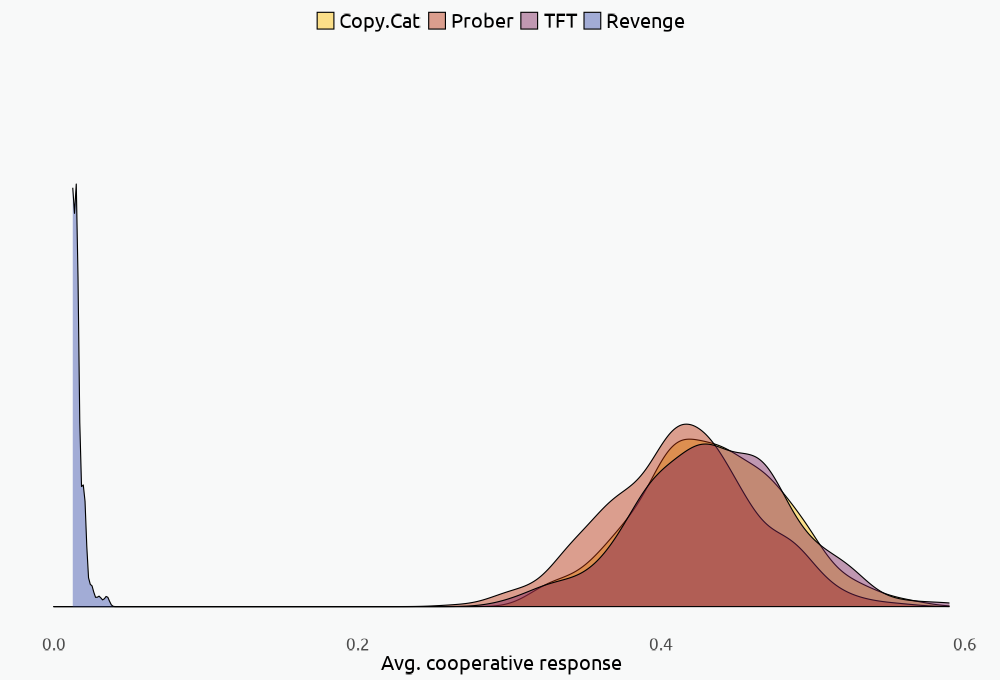
The cooperative response plot shows that, on average, the tit–for–tat algorithm cooperates more often than the vengeful and the prober algorithms, but just as much as copy.cat5.
5 I used the Wilcoxon rank sum test to compute the difference in medians and check if the algorithm distributions are stochastically equivalent. It’s not clear whether the prober algorithm is equivalent to tit.for.tat, but the test shows a statistically significant difference in the algorithms’ median cooperative responses.
Code
wilcox_gt <- mean_df |>
  filter(kind == c("TFT","Prober")) |>
  pivot_longer(cols = -kind, names_to = "vars",
               values_to = "values") |>
  group_by(vars) |>
  summarize(
  Estimate = wilcox.test(values~kind, conf.int = T)$estimate,
  Sig. = wilcox.test(values~kind, conf.int = T)$p.value
  ) |>
  gt() |>
  tab_header(
    title = md("*Comparison of Tit×Tat and Prober cooperative responses*")
    ) |>
  cols_label(vars = md("**Estimate**"),
             Estimate = md("**Difference in estimate**"),
            Sig. = md("**p-value**")) |>
  cols_align(align = "center") |>
  opt_table_font(font = google_font("EB Garamond"),
                 weight = 400,style = "plain", add = TRUE) |>
  tab_style(style = cell_text(font = google_font("Ubuntu")),
            locations = cells_body()) |>
   tab_options(column_labels.font.weight = "bold",
              row_group.font.weight = "bold") |>
  data_color(rows = everything(),
             palette = "#f9f9f9")

wilcox_gt| Comparison of Tit×Tat and Prober cooperative responses | ||
|---|---|---|
| Estimate | Difference in estimate | p-value |
| Median | -2.38e-05 | 0.0451 |
Axelrod believed that, on average, “nice” algorithms would perform better than “ mean and deceitful” ones like exact.revenge and prober, and we can clearly see that our most vengeful algorithm performs poorly on the cooperative front, with a mean cooperation of .0055 per game, about once per game.
Based on the algorithm’s cooperative response we can then visualize and compute the final score distribution (in total points) for each player after 500 games of 200 rounds each. We’ll see that, by defecting often and without provocation, the second player typically scores much higher than player 1. However, when player 2 chooses to not betray without provocation or imitate the first’s player current choices both players end up with higher and approximately equal scores. Because of this willingness to cooperate, according to Axelrod, the nice algorithms tend to be more conducive to cooperation and less prone to conflict.
Code for data manipulation & plots
test2 <- comp.alg(c(exact.revenge, prober),
                 iter = 500,
                 rounds = 200,
                 prob = c(.345, .231),
                 choice = 0,
                 default = .10) |> rename("R.P1" = "A1P1",
                                          "R.P2" = "A1P2",
                                          "Pr.P1" = "A2P1",
                                          "Pr.P2" = "A2P2")

perf_df <- cbind(test,test2) |> pivot_longer(cols = everything(),
               names_to = c("Algorithm", "Player"),
               names_pattern = "([^.]+)\\.(P\\d)",
               values_to = "Score") |>
  mutate(Algorithm = case_when(
           Algorithm == "R" ~ "Revenge",
           Algorithm == "Pr" ~ "Prober",
           Algorithm == "CC" ~"Copy.Cat",
           Algorithm == "TFT" ~ "Tit×Tat",
           TRUE ~Algorithm
         ),
         Algorithm = factor(Algorithm),
         Player = factor(Player)) |>
  arrange(Algorithm, Player) |>
  group_by(Algorithm, Player)

#> str(perf_df)

 p1 <- ggplot(perf_df, aes(Score, fill= Player)) +
  geom_density(alpha = .45) +
  labs(title = NULL,
       x = NULL,
       y = NULL) +
  scale_fill_manual(values = clrs)


 p2 <- ggplot(perf_df, aes(Score, fill= Algorithm)) +
  geom_density(alpha = .45) +
  labs(title = NULL,
       x = "Score",
       y = NULL) +
  scale_fill_manual(values = clrs)

#> p1/p2
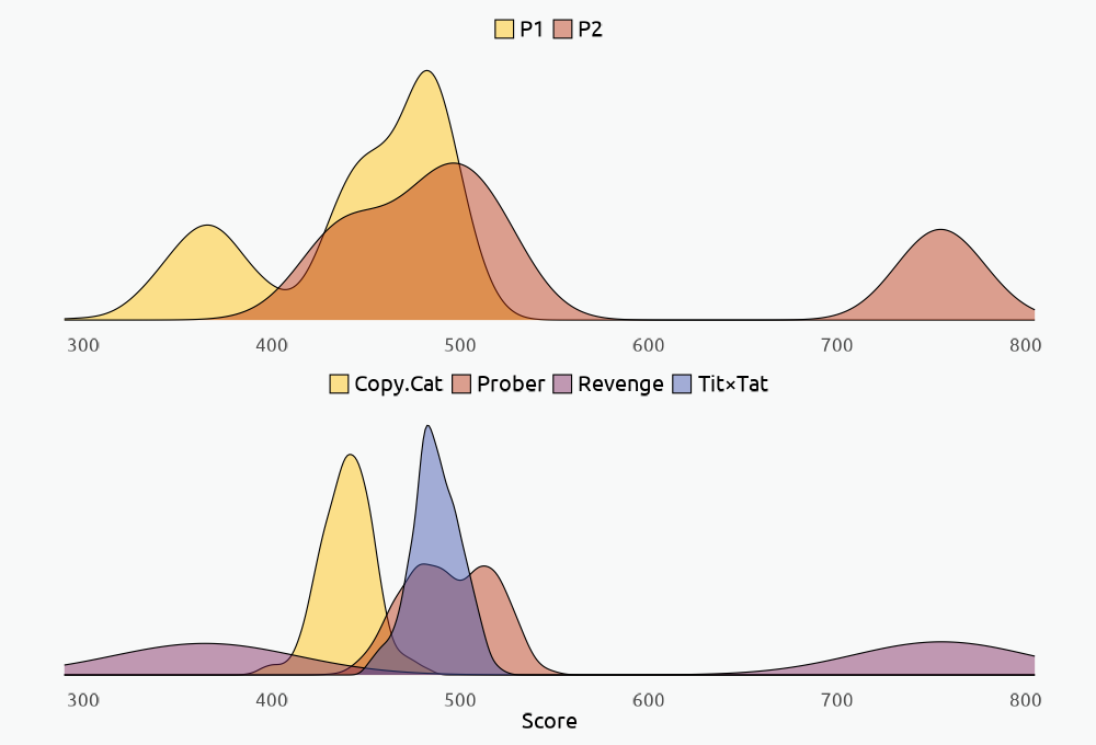
These two plots show the performance of both players and the four algorithms, and we can see that the most extreme results are obtained using the exact.revenge algorithm. The density curves for this algorithm are touching the extremes on the left and right, showing that one player will always under perform while the other one, typically the second one, will outperform his opponent. This algorithm is a “sneaky” one because player 1 is not able to confidently predict his opponent’s moves. Regardless of his choice, after the first betrayal, player 2 will never cooperate again.
To my surprise, the prober algorithm returned a more favorable score for player 2 than the tit.for.tat or the copy.cat algorithm; however, the nice algorithms always favored both players, not just player 2.
Code
 sumperf_gt <- perf_df |> summarise(Score = mean(Score)) |>
  arrange(Algorithm) |>
  as_tibble() |> gt() |>
  tab_header(title = md("*Average Player Score by Algorithm*")) |>
  cols_label(Algorithm = md("**Algorithm**"),
             Player = md("**Player**"),
            Score = md("**Score**")) |>
  opt_table_font(font = google_font("EB Garamond"),
                 weight = 400,style = "plain", add = TRUE) |>
  tab_style(style = cell_text(font = google_font("Ubuntu")),
            locations = cells_body()) |>
   tab_options(column_labels.font.weight = "bold",
              row_group.font.weight = "bold") |>
  data_color(rows = everything(),
             palette = "#f9f9f9") |>
  opt_interactive(use_compact_mode = TRUE, use_highlight = TRUE)

 sumperf_gt
Average Player Score by Algorithm
Nevertheless, regardless of which algorithm we used, player 1’s score is, on average, lower than player 2, even if the nice algorithms tend to equalize the scores and may result in less conflict as Axelrod described.
practical implications
Among all the algorithms submitted to Axelrod, the top performer was Tit–for–tat because it was “nice”. Algorithms that always betrayed or were “sneaky” were more likely to end up in a state of conflict. Our custom algorithms also showed this behavior, both players thrived when cooperation was a priority for one of the players. In our case, the tit.for.tat algorithm outperformed others in this regard even if it didn’t achieve the maximum number of points like the exact.revenge algorithm.
Based on this short experiment, we can conclude that cooperation is better than conflict for all parties involved. We should accept betrayal and quickly forgive to attain a more favorable outcome. We shouldn’t be “pushovers” and always cooperate regardless of our opponent’s actions. Instead,we should be just and merciful, meting out justice when previously betrayed but extending mercy when our opponent doesn’t deserve it.
Here are some rules for strategic cooperation derived from our algorithms:
- Avoid unnecessary conflict by cooperating as long as your opponent does.
- If your opponent betrays you without provocation— respond in kind…once.
- Then forgive the betrayal, and cooperate again.
- Be clear and predictable so your opponent knows how you act and can plan accordingly.
Citation
For attribution, please cite this work as:
Monteagudo, JP. 2024. “The Iterated Prisoners’ Dilemma.”
July 3, 2024. https://doi.org/10.59350/gyxmw-enh88.