
The programs (together with their sources and the data sets used in the book) are available on floppy disks by writing to the authors.
cluster analysis
The goal of cluster analysis is to find groups in the data. Sometimes groups are naturally present in the data, and sometimes they are artificially created. These groups are called clusters and the analyst tries to discover them using statistical techniques. Cluster analysis establishes the groups to which several data points belong. It does not assign objects to groups that have been defined in advance.
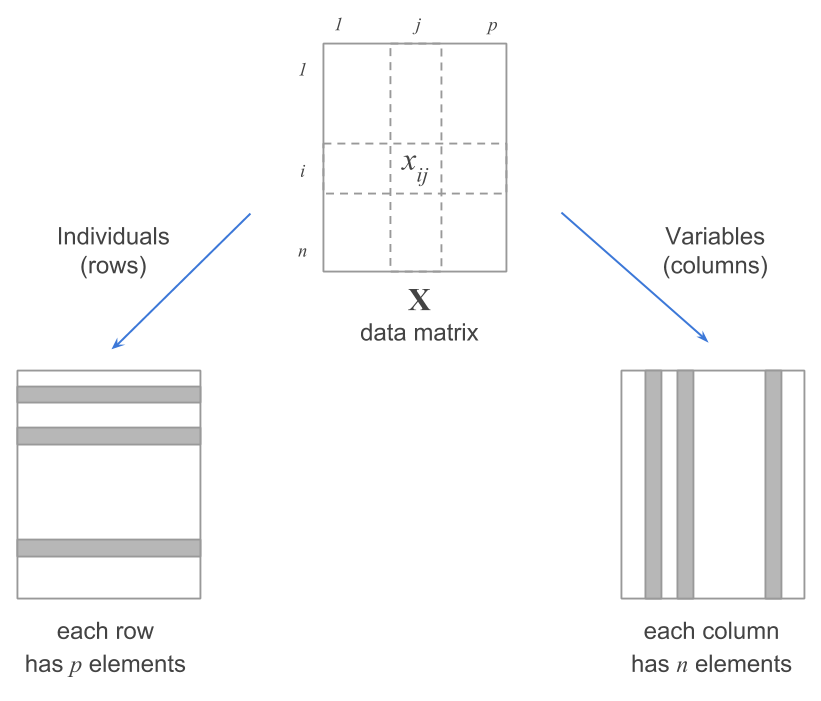
The data are organized in tabular form in one of two ways. The first places each object in a row and each measured attribute in a column. Think of a group of people and their heights, weights, and ages. Each row represents a person, and the columns show their measurements. This is called an n-by-p matrix.
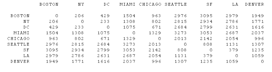
The second places the objects in columns and rows. This is called a n-by-n matrix. Think of a group of cities for which we want to compare driving distances. Each city would be assigned a row and a column, and the intersection of the row and column would contain the driving distance between the two cities.
Before the clusters are identified, the data needs to be transformed1 to make them suitable for cluster analysis. Why? Because depending on the units of our measurements, the grouping may be interpreted differently. For example, if we have a data set with the heights of people in centimeters and weights in kilograms, the clustering may be different than if we had the heights in inches and weights in pounds.
1 The aim of transforming the data is to assign equal weights to all variables, thus getting rid of relative weights across the board to achieve an objective comparison. However, some variables will, at times, be more important than other, and this matter should not be disregarded.
Code
persons_data <- data.frame(
  Name = c("Alice", "Bob", "Charlie", "Diana", "Eve"),
  Weight = c(15,49,13,45,85),
  Height = c(95, 160, 90, 160, 180)
)

person_table <- persons_data |>
  tinytable::tt(digits = 3,
     caption = "Weight and Height of Five People, expressed in Kilograms and Centimeters",
     theme = "spacing"
    ) |>
  style_tt(align = "lcc",
           boostrap_class = "table table-hover")

person_table| Name | Weight | Height |
|---|---|---|
| Alice | 15 | 95 |
| Bob | 49 | 160 |
| Charlie | 13 | 90 |
| Diana | 45 | 160 |
| Eve | 85 | 180 |
Code
par(family = "serif")
plot.new()
plot.window(
  xlim = c(0,90),
  ylim = c(0,200)
            )

points(persons_data$Weight, persons_data$Height, pch = 19, col = "gray50")
text(persons_data$Weight, persons_data$Height, labels = persons_data$Name, pos = 3, cex = 1.10)
axis(1, at = seq(0, 90, 15), tcl = -0.05, labels = TRUE)
axis(2, at = seq(0, 200, 20), tcl = -0.05, labels = TRUE, las=2)
mtext("Weight (kg)", side = 1, line = 2.5, at = 80, font = 2, cex = 1.2)
mtext("Height (cm)", side = 2, line = -6.5, at = 200,las = 2, font = 2, cex = 1.2)

pounds <- persons_data$Weight * 2.20462
inches <- persons_data$Height * 0.393701

plot.new()
plot.window(
  xlim = c(0,200),
  ylim = c(0,120)
            )

points(pounds,inches, pch = 19, col = "gray50")
text(pounds, inches, labels = persons_data$Name, pos = 3, cex = 1.10)
axis(1, at = seq(0, 200, 15), tcl = -0.05, labels = TRUE)
axis(2, at = seq(0, 90, 15), tcl = -0.05, labels = TRUE, las=2)
mtext("Weight (lbs)", side = 1, line = 2.5, at = 180, font = 2, cex = 1.2)
mtext("Height (in)", side = 2, line = -6.5, at = 90,las = 2, font = 2, cex = 1.2)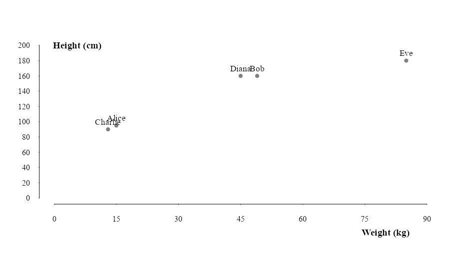
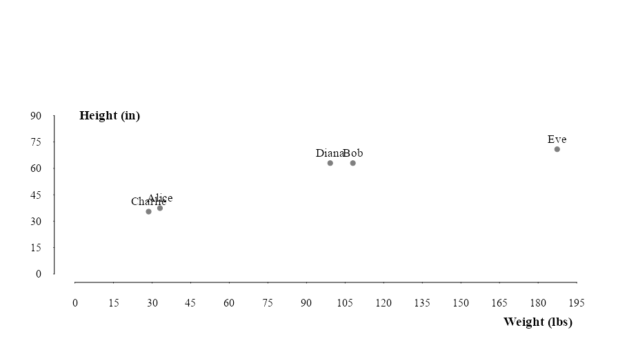
Notice in this example that the first plot offers a clearer natural partition of groups than the second plot. We can see that Charlie and Alice are most likely children while Diana, Bob and Eve are adults. The height of a person gives a better indication of adulthood than weight. So when we plot height in inches againts weight in pounds, weight becomes the dominant variable and the distinction between clusters become less clear.
variable selection
What variables shall we choose? Should we standardize or use the raw data? To answer the first question, let me say that we should use variables that contain relevant information about each object. Sometimes these decisions will come down to common sense or expert knowledge. For example,using phone numbers, license plates,favorite colors,country flags,a variable where all rows are missing, etc., for each object is useless because none of these variable provide relevant information about the objects they represent.
The negative side effect of using such variables is that are clusters will fail to form because of the randomness introduced by these “trash” variables. The soultion here is to assign a weight or zero or remove them from our data.
To answer the standardization question– we should standardize the data prior to calculating disances if we think the units chosen were not appropriate or well thought-out measures and we’d like to assign weights to the variables. Additionally, if, based on prior knowledge, we would like to apply certain weights to each variable, we can standardize or just chnage the measurement units. However, if we’d like to keep the data intact because the measurements are meaningful, don’t standardize.
In our particular example, we’d like to avoid the dependence on measurement units, wso we standardize the data to convert the original measurements to uniteless variables.
\[ \begin{split} m_{f} = \frac{1}{n} \sum_{x = 1}^{n}x_{f} \\ std_{f} = \sqrt{\frac{1}{n-1} \sum_{x = 1}^{n} (x_{f} - m_{f}^2)} \\ \end{split} \]
However,because the mean and standard deviation are affected by outliers, it is better to use the mean absolute deviation to calculate the standardized values. \[ \begin{split} s_{f} = \frac{1}{n} \sum_{x = 1}^{n}|x_{f}-m_{f}| \\ z_{if} = \frac{x_{if} - m_{f}}{s_{f}} \end{split} \] Now our data have mean of zero and a mean absolute deviation of 1. We can begin using the standardized data instead of the original2.
2 If every variable is expressed in the same units, there’s no need for standardization.
distance metrics
Next, we find the distances between the objects to quantify their degree of dissimilarity. All distance function must satisfy the following requirements:
\[ \begin{split} d(i,j) \geq 0 \\ d(i,i) = 0 \\ d(i,j) = d(j,i)\\ d(i,j) \leq d(i,h) + d(h,j)\\ \end{split} \] So distances must be nonnegative numbers3. The distance of an object to itself must be zero. The distance between to objects is the same regardless of the order in which they are compared. And lastly, the distance between two objects is always less than or equal to the sum of the distances between the two objects and a third object.
3 by the same token, we can only calculate distances for non-missing object pairs. \(n\) is the total number of non-missing objects
euclidean distance
\[ \begin{split} d(i,j) = \sqrt{\sum_{n=1}^{p} (x_{in} - x_{jn})^2} \end{split} \]
manhattan distance
\[ \begin{split} d(i,j) = \sum_{n =1}^{p} |x_{in}-x_{jn}| \end{split} \]
minkowski distance
This is a generalization of the Euclidean and Manhattan metric, where \(q\) is any real number larger than 1. \[ \begin{split} d(i,j) = {\sum_{n =1}^{p}|x_{in}-x_{jn}|^\frac{1}{q}} \end{split} \]
weighted euclidean distance
A slight variation on the Euclidean distance where each variable receives a weight4 according to its relative importance. \[ \begin{split} d(i,j) = \sqrt{wn\sum_{n=1}^{p} (x_{in} - x_{jn})^2} \end{split} \]
4 giving a variable a weight of 2 is the same thing as using it twice
Here’s the Euclidean and Manhattan distances for our previous example:
Code
euclidean <- dist(persons_data[,2:3],
                  method = "euclidean",
                  diag = FALSE,
                  upper = FALSE) |>
  as.matrix()

# Keep only the lower triangle (excluding diagonal)
euclidean[upper.tri(euclidean, diag = FALSE)] <- NA

  euclidean <- euclidean |>
    as.data.frame() |>
    dplyr::rename(
      Alice = 1,
      Charlie = 2,
      Diana = 3,
      Bob = 4,
      Eve = 5
    )

rownames(euclidean) <- persons_data$Name

euclidean_table <- euclidean |>
  tinytable::tt(
    digits = 2,
    caption = "Euclidean Distance of Unstandardized Weight(kg) and Height(cm) for five people",
     theme = "spacing",
    rownames = TRUE
    ) |>
  style_tt(align = "c",
           boostrap_class = "table table-hover")

euclidean_table| rowname | Alice | Charlie | Diana | Bob | Eve |
|---|---|---|---|---|---|
| Alice | 0 | ||||
| Bob | 73.4 | 0 | |||
| Charlie | 5.4 | 79 | 0 | ||
| Diana | 71.6 | 4 | 77 | 0 | |
| Eve | 110.1 | 41 | 115 | 45 | 0 |
Code
manhattan <- dist(persons_data[,2:3],
                  method = "manhattan",
                  diag = FALSE,
                  upper = FALSE) |>
  as.matrix()

manhattan[upper.tri(manhattan, diag = FALSE)] <- NA

  manhattan <- manhattan |>
    as.data.frame() |>
    dplyr::rename(
      Alice = 1,
      Charlie = 2,
      Diana = 3,
      Bob = 4,
      Eve = 5
    )

rownames(manhattan) <- persons_data$Name

manhattan_table <- manhattan |>
  tinytable::tt(
    digits = 2,
    caption = "Manhattan Distance of Unstandardized Weight(kg) and Height(cm) for five people",
     theme = "spacing",
    rownames = TRUE
    ) |>
  style_tt(align = "c",
           boostrap_class = "table table-hover")

manhattan_table| rowname | Alice | Charlie | Diana | Bob | Eve |
|---|---|---|---|---|---|
| Alice | 0 | ||||
| Bob | 99 | 0 | |||
| Charlie | 7 | 106 | 0 | ||
| Diana | 95 | 4 | 102 | 0 | |
| Eve | 155 | 56 | 162 | 60 | 0 |
Notice that regardless of the distance metric used, the groups are comparably the same. However, this matrix doesn’t clearly show the cluster structure of our data like the bivariate scatterplot. Nevertheless, this is the matrix our clustering algorithm works with.
dissimilarities
We refer to the many possibilities that can function as a distance matrix as dissimilarities. Dissimilarity coefficients must be nonnegative numbers that are small when \(i\) and \(j\) are near to each other and large when they are very different. Dissimilarities can be computed for binary, nominal, ordinal, interval, and continuous variables, or a combination of these.
One such dissimilarity index is Pearson’s product-moment coefficient5 or Spearman’s rho. These correlation coefficients can be converted to dissimilarities
5 . Pearson’s r looks for a linear relationship between two variables while Spearman’s rho looks for a monotonic relationship, not a linear one.
\[ \begin{split} R(f,g) = \frac{\sum_{i=1}^{n} (x_{if} - m_{f})(X_{ig} - m_{g})}{\sqrt{\sum_{i=1}^{n} (x_{if} - m_{f})^2} \sqrt{\sum_{i=1}^{n} (x_{ig} - m_{g})^2}} \\ \\ \\ d(f,g) = (1 - R(f,g))/2 \end{split} \] Using the previous formula for \(d(f,g)\), we see that variables with a high positive correlation will have a dissimilarity coefficient close to zero while variables with a high negative correlation will be very dissimilar. Another formula that’s available is the following:
\[ \begin{split} d(f,g) = 1 - |R(f,g)| \end{split} \]
By adding a third variable, Year, to represent each person’s birth year, we can compute a dissimilarity matrix that shows how different or distant is the birth year from the weight and height of each person. The resulting matrix would help us determine how many groups and which members to include in each group.
Code
persons_df_with_year <- persons_data |>
  dplyr::mutate(
    Year = c(2018,
             1999,
             2020,
             1889,
             2003),
    .before  = 2
  )

year_table <- persons_df_with_year |>
  tinytable::tt(digits = 0,
                caption = "Birth Year, Weight(kg) and Height(cm) of Five People, expressed in Kilograms and Centimeters",
                theme = "spacing") |>
  tinytable::style_tt(align = "lccc")

year_table| Name | Year | Weight | Height |
|---|---|---|---|
| Alice | 2018 | 15 | 95 |
| Bob | 1999 | 49 | 160 |
| Charlie | 2020 | 13 | 90 |
| Diana | 1889 | 45 | 160 |
| Eve | 2003 | 85 | 180 |
Let’s come up with the dissimilarity matrix for these data using the two dissimilarity formulas we’ve looked at.
Code
cluster_dissimilarity <- function(x,
                                  dissimilarity_method = c("halved","absolute"),
                                  correlation = c("pearson","spearman")){

  # Stop if not a matrix or data frame
  stopifnot(is.matrix(x) || is.data.frame(x))

  # If function args don't match these, stop.
  dissimilarity_method <- match.arg(dissimilarity_method)
  correlation <- match.arg(correlation)

  # Just in case any columns are strings or factors,
  # convert to numeric to compute correlation
  x <- data.matrix(x)

  cor_coeff <- cor(x,method = correlation)

  dissimilarity_coeff <- switch(dissimilarity_method,
     "halved"  = (1 - cor_coeff)/2,
     "absolute"= 1 - abs(cor_coeff)
  )

  # remove redundant correlations
  dissimilarity_coeff[upper.tri(dissimilarity_coeff, diag = FALSE)] <- NA

  return(dissimilarity_coeff)
}

pearsons_dissimilarity <- cluster_dissimilarity(persons_df_with_year,
                              dissimilarity_method = "halved",
                              correlation = "pearson") |>
  # Need to convert to df before creating to tinytable
  as.data.frame()

# Add rownames to the data frame
rownames(pearsons_dissimilarity) <- c("Name","Year","Weight","Height")

  pearsons_table <- pearsons_dissimilarity |>
    tinytable::tt(digits = 3,
                caption = "Dissimilarity Coefficients Between Year, Weight(kg) and Height(cm) Using Pearson's r and the Halved Dissimilarity Formula",
                theme = "spacing",
                rownames = TRUE) |>
tinytable::style_tt(align = "lcccc")| rowname | Name | Year | Weight | Height |
|---|---|---|---|---|
| Name | 0 | |||
| Year | 0.702 | 0 | ||
| Weight | 0.135 | 0.602 | 0 | |
| Height | 0.176 | 0.728 | 0.0321 | 0 |
| Name | Year | Weight | Height |
|---|---|---|---|
| 0 | |||
| 0.597 | 0 | ||
| 0.27 | 0.796 | 0 | |
| 0.352 | 0.545 | 0.0642 | 0 |
r packages
cluster
Citation
For attribution, please cite this work as:
Monteagudo, JP. 2025. “Cluster Analysis.” March 6, 2025. https://www.jpmonteagudo.com/blog/2025/03.